Theory:
In digital control systems, specific dynamic characteristics can be achieved by appropriate placement of closed-loop poles in the z-domain.
One such characteristic is the deadbeat response, in which the system output reaches its final value in the minimum possible number of sampling periods and remains there without oscillations or steady-state error.
A deadbeat response refers to a discrete-time system output that becomes equal to the desired final value in a finite number of samples, typically equal to the system order.
For an 𝑛-th order system, the output ideally settles at the final value in exactly 𝑛 sampling instants and remains constant for all subsequent samples.
This behavior is unique to discrete-time systems and is achieved by placing all closed-loop poles at the origin in the z-plane (i.e., 𝑧 = 0).
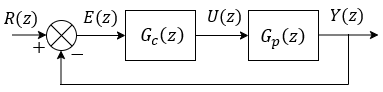 Fig.1. Block Diagram of Deadbeat Control System
Consider a discrete-time system represented by the transfer function:
$$ G_p(z) = \frac{Y(z)}{R(z)} = \frac{b_0+b_1 z^{-1}+...+b_m z^{-m}}{1+a_1 z^{-1}+...+a_n Z^{-n}} \tag{1} $$
A deadbeat response is achieved by designing the controller as:
$$ G_c(z) = \frac{1}{G_p(z)} \frac{T(z)}{1-T(z)}\tag{2} $$
This means all closed-loop poles are placed at the origin, ensuring that the system's transient response dies out in exactly 𝑛 samples.
The number of poles at the origin directly determines the number of sampling instants the system requires to settle.
Placing 𝑛 poles at 𝑧 = 0 introduces 𝑛 dynamic modes, each of which decays in one sample. Therefore, the system output remains zero until sample 𝑘 = 𝑛, at which point it jumps to the final value and remains there.
For an 𝑛-th order system with all poles at the origin, the transfer function has the form:
$$ T(z) = \frac{1}{z^n} \tag{3} $$
Thus, each pole at the origin contributes one sample of delay, and the full system settles in 𝑛 steps, where 𝑛 is the system order.
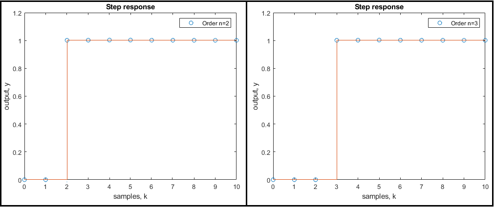 Fig.2. Deadbeat response of an all digital control system for unit step input
Linear time invariant system may be represented in state space form by the following equations:
State equation:
$$ \dot{x}(t)=A x(t)+B u(t) \tag{4a} $$
Output equation:
$$ y(t)= C x(t) \tag{4b} $$
Deadbeat Control design:
A deadbeat controller is one where the system's output reaches its desired value in the smallest number of steps (the so-called "deadbeat time" or "deadbeat response").
This is achieved by designing the control law such that the poles of the closed-loop system lie at the origin.
The discrete-time state space model with feedback can be written as:
State equation:
$$ {x}[k+1]=F x[k]+g u[k] \tag{5a} $$
Output equation:
$$ y[k] = C x[k] \tag{5b} $$
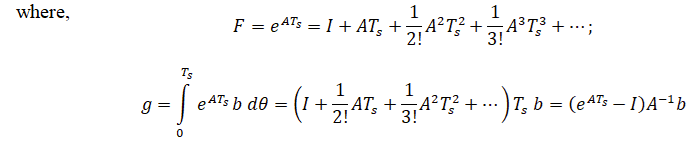
where,
x[
k] is state vector,
y[
k] is output vector,
u is input or control vector,
F is system matrix,
g is input matrix,
C is output matrix,
Ts is the sampling time.
The control input is typically given by:
$$ u[k] = - K x[k] + r[k] \tag{6} $$
where,
K is the state feedback gain matrix,
r[
k] is the reference signal.
State feedback design for deadbeat response:
The goal of deadbeat control is to place the poles of the closed-loop system at the origin of the z-plane, i.e., all the eigenvalues of (
F -
gK) should be at zero. This ensures the system reaches the equilibrium state (desired state) as quickly as possible.
For a discrete-time system, the characteristic equation of the closed-loop system is derived from the state-space model with the feedback gain
K. The poles of the system are determined by the eigenvalues of (
F -
gK).
Controllability: The system must be controllable for a deadbeat design to be possible. Controllability ensures that it's possible to drive the system from any initial state to any desired state using the available inputs.
Pole Placement: To achieve a deadbeat response, place the poles of the closed-loop system at the origin. This requires solving for the feedback gain matrix
K that ensures that all eigenvalues of the matrix (
F -
gK) are zero.
Solve for
K such that the eigenvalues of (
F -
gK) are at the origin.
• Determinant of (
F -
gK) = 0.
• Trace of (
F -
gK) = 0.
State feedback design:
A necessary and sufficient condition for arbitrary pole placement is that the pair (
F,
g) must be controllable.
Control input:
$$ u[k]= - K x[k] \tag{7} $$
where,
K is the state feedback gain vector,i.e.,
$$ K = [k_1 \ k_2 \ ... \ k_n] $$
With this control input, the closed loop system is as follows:
$$ x[k+1]=(F-gK) x[k] $$
The characteristic equation of the closed loop system is,
$$ |zI-(F-gK)|=0 $$
For
nth order system, the characteristic equation is,
$$ z^n + \alpha_n z^{n-1} + \alpha_{n-1} z^{n-2} + ... + \alpha_1=0 \tag{8} $$
where,
αi for
i=1, 2, ..., n depends on
F, g, K.
The desired closed loop poles (in s domain) are
P1,
P2,
P3, ... ,
Pn.
The desired closed loop poles (in z domain) are
Pz1,
Pz2,
Pz3, ... ,
Pzn.
Then the desired characteristic equation is:
$$ (z-{P_z}_1)(z-{P_z}_2)(z-{P_z}_3)...(z-{P_z}_n)=0 \tag{9} $$
The required state feedback gain (
K) vector elements are obtained by comparing the matching coefficients of (5) and (6).
State Space Model of Mechanical System:
Consider the mechanical system shown in Fig. 3. Assume that the system is linear. The external force
u(
t) is the input to the system, and the displacement
y(
t) of the mass is the output.
The displacement
y(
t) is measured from the equilibrium position in the absence of the external force. This system is a single-input, single-output system.
 Fig.3. Mechanical System
where,
m is mass,
b is damping friction,
k is the spring constant,
y is the displacement (output) and
u is the external force.
The system equation is:
$$ m\ddot{y} + b \dot{y} + k y = u \tag{10} $$
State Space form of the Mechanical system:
The State Space form:
Continuous State Space form:
$$ \begin{bmatrix} \dot{x}_1(t) \\ \dot{x}_2(t) \end{bmatrix} = \begin{bmatrix} 0 & 1 \\ -\frac{k}{m} & -\frac{b}{m} \end{bmatrix} \begin{bmatrix} x_1(t) \\ x_2(t) \end{bmatrix} + \begin{bmatrix} 0 \\ \frac{1}{m} \end{bmatrix} u(t) $$
$$ y(t) = \begin{bmatrix} 1 & 0 \end{bmatrix} \begin{bmatrix} x_1(t) \\ x_2(t) \end{bmatrix} \quad \tag{11} $$
where,
x1 is the displacement,
x2 is the velocity,
u(t) is the external force,
y(t) is the output.
Discrete State Space form:
$$ \begin{bmatrix} x_1 [k+1] \\ x_2 [k+1] \end{bmatrix} = \begin{bmatrix} 1 & T_s \\ -\frac{k T_s}{m} & 1-\frac{b T_s}{m} \end{bmatrix} \begin{bmatrix} x_1 [k] \\ x_2 [k] \end{bmatrix} + \begin{bmatrix} \frac{{T_s}^2}{2m} \\ \frac{T_s}{m} (1-\frac{b T_s}{2m}) \end{bmatrix} u[k] $$
$$ y [k] = \begin{bmatrix} 1 & 0 \end{bmatrix} \begin{bmatrix} x_1[k] \\ x_2[k] \end{bmatrix} \quad \tag{12} $$