
Go through the instructions to perform the experiment Click Here
Aim:
To understand the pathloss prediction formula.Objective:
- Calculation of received signal strength as a function of distance of separation, antenna height and carrier frequency.
- To understand the impact of :-
- Transmitter Power,
- Pathloss exponent,
- Carrier frequency,
- Receiver antenna height,
- Transmitter antenna height.

Exp-1: Understand the pathloss prediction formula
Aim:
To understand the pathloss prediction formula.Objective:
- Calculation of received signal strength as a function of distance of separation between transmitter and receiver.
- To understand the impact of the following parameters on received signal strength.
- Transmitter Power,
- Pathloss exponent,
- Carrier frequency,
- Receiver antenna height,
- Transmitter antenna height.
Theory for Experiment 1: Understand the pathloss prediction formula
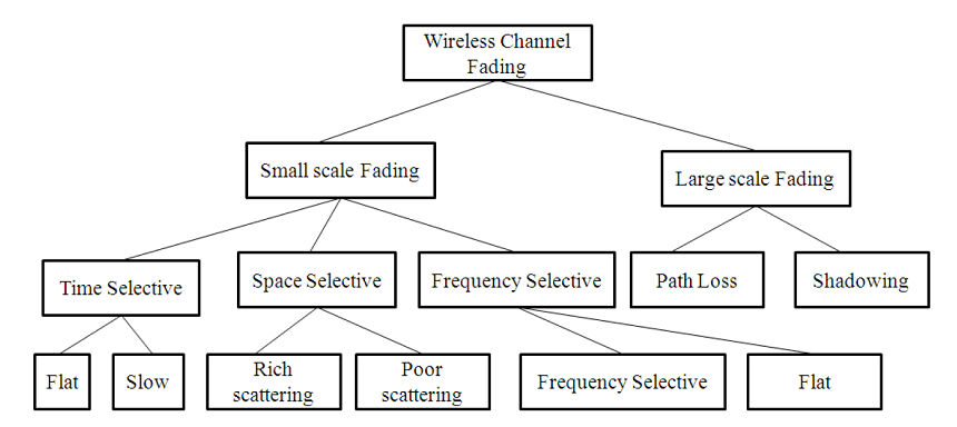
The design of a communication system involves selection of values for several parameters. One of the important parameter is the transmit power. Higher transmit power ensures large allowable separation distance between the transmitter (Tx) and receiver (Rx). Of course the loss in signal power per unit distance depends on the properties of the medium. In case of wireless communication on one hand it is desired to have a very large coverage (large allowable separation between Tx and Rx) on the other hand it is also desired that co-channel interference be as low as possible. An understanding of the large scale propagation effects is very important for design of suitable communication system. In terrestrial mobile communication system, electro-magnetic wave propagation is affected by reflection, diffraction and scattering. These lead to dynamic variation of signal strength as a function of time, frequency, distance of separation, antenna height, antenna configuration, local scattering environment etc. Propagation models are necessary in order to predict the received signal strength for a given set of parameters as mentioned above. These models can be broadly considered under:-
- Large scale Fading Model.
- Small Scale Fading Model.
1.1 Large Scale Fading:-
Large Scale Fading is dealt by propagation models that predict the mean received signal strength for an arbitrary transmitter receiver separation. The large scale fading model gives such an average with measurements across 4`lambda` to 40`lambda`, where `lambda` is the wavelength. This is useful for estimating coverage area. Large Scale fading can be broadly classified as:-
- Path Loss.
- Shadowing.
Large scale fading is heavily affected by power dissipation and effects of the propagation channels. The models assume some path loss at a given distance between Tx and Rx i.e. there is no shadowing. It is useful in getting a quick estimate of the average signal strength, hence the coverage. These models are used for prediction of signal variation across 100m-1000m.
There have been ray tracing methods which are complicated and are useful for static scenarios. In case of dynamic scenarios statistical models are used. A statistical model ensures that the statistical properties of the numbers generated using the model matches the recorded values.
We begin with Friis Free space propagation loss. The received power at a distance'd' is given by.
`P_r(d)= (P_tG_tG_rlambda^2)/((4lambda^2d^2l))` where `G =(4PiA_e)/ lambda^2`
- `P_t=`Transmitter Power.
- `P_r(d)=`Received power at a distance'd'.
- `G_t=`Transmit antenna power gain.
- `G_r=`Received antenna power gain.
- `lambda=`Wavelength.
- `A_e=`Effective aperture related to the physical size of antenna.
- `L>=1`System loss factor not related to propagation .
Transmission line , Filter losses, Antenna loss etc . - `D=T_x-R_x` separation distance.
`P_r`decrease as square of distance 20 dB/ decade.
Path loss gives a measure of signal attenation. It is usually measured in dB.It is defined as a difference between the transmitted antenna gains.
The path loss for free space model is
PL(dB)`=10log_10(P_t/P_r)` `=-10log_10[(G_tG_rlambda^2)/((4pi)^2d^2)]`
It may be remembered that Friis free space model is valid for 'd' in the far field of the transmission antenna. The far field / Fraunhofer region is beyond the far field distance, where `d_f=(2D^2)//lambda`.
It is related to the largest linear dimension of the antenna aperture and carrier wavelength. d is the largest linear distance of the antenna. `d_f`>>d and `d_f`>>`lambda` then it is the far field region. For path loss models 'd'
can't be 0.
Therefore a close in distance is used which is known as the received power reference point .Thus `P_r(d)` for `d>d_0` may be reference to `P_r(d_0)` where `P_r(d_0)` may be predicted from Friis free space propagation
loss model. It may also be obtained from measurements by using average of several recordings at distance `d_0`. The distance `d_0`>>`d_f` but `d_0` is sufficiently smaller than practical BS-MS distance.
`P_r(d)=P_r(d_0)*(d_0//d)^2`, `d>=d_0>=d_f`
Usually received signal strength is measured in dBm or dBw.
`P_r(d)`dBm`=10log_10((P_rd_0)/(10^-3omega))+20log_10(d_0/d)` , `d>=d_0>=d_f`
Where `P_r(d_0)` is in watt.
The Value `d_0` in 1-2 GHz.
~1m for indoor condition.
~100m`//`1km for indoor condition.
The received power predicted by path loss models is influenced by
Reflection: Reflection occurs when the propagation waves impinge on objects with dimension larger than `lambda`.
Diffraction: Diffraction is caused by sharp irregularities in the path of radio waves. It leads to development of secondary wave fronts, bending of waves. It is caused by objects which are in order in `lambda`. It depends on geometry of the objects, amplitude, phase and polarization of incident waves.
Scattering: Scattering is caused by objects which are smaller than `lambda`.
Using the famous 2-Ray propagation model [Ref(Rappaport)] . It can be shown that when a transmitter at height `h_t` transmit with power `P_t` having antenna gain `G_t` the receiver signal power at the receiver located at height `h_r` using an antenna with gain `G_r` and located at a distance 'd' from the transmitter given by
`P_r= P_tG_tG_r((h_t^2h_r^2)/d^4)`, for d>> `sqrt(h_th_r)`
When `theta_Delta` is small( <0.3rads) `sin(theta_Delta//2)``~(theta_Delta/2)`
`theta_Delta/2~~(2pih_th_r)/(lambdad)` `->d>(20pih_th_r)/(3pi)~~(20h_th_r)/lambda`
For all above range of d,
`E_(TOT)~~``(2E_0d_0)/d 2pih_th_r/(lambdad)~~``k/d^2 V//m`
k is related to `E_0`,antenna heights and `lambda`
Power received is proportional to square of electric field.
Therefore received power from transmitter at a distance d is
`P_r= P_tG_tG_r((h_t^2h_r^2)/d^4)`, for d>> `sqrt(h_th_r)`
Power deceases with fourth power d `->` 40dB`//`decade
The pathloss for the 2 Ray model is given by
`PL(dB)=40logd-(10logG_t+10logG_r+20logh_t+20logh_r)`
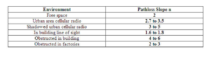
In general the PL and `d^(-n_r)` is the pathloss exponent. The value of `n_p` can be obtained analytically/emperically.
Emperically models have the advantage of taking all factors into account (both known and unknown).It is based on actual field measurement.
Its disadvantage is that it is valid for only the measured frequency and location.
Generally
`bar(PL(dB))=``bar(PL(d_0))+10n_plog(d/d_0)`
Pathloss models are defined for:
- Indoor office test environment
`PL=37+30log_10(R)+(18xx3xxn^((n+2)/((n+1)-0.46)))` [dB]
- R=transmitter-receiver Seperation.
- n=no. of floor in the path.
- L shall in all cases > free space loss.
- Outdoor to indoor and pedestrian testr environment(base model)
`PL=40log_10(R)+30log_10(f)=49` [dB]
- R= base station to mobile station deviation [Km],
- f= carrier frequency [MHz], reference 2000 MHz.
- Vehicular test environment
`PL=40(1-4xx10^-3xxDeltah_b)log_10(R)-18log_10(Deltah_b)+21log_10(f)+80` [dB]
- R= base station to mobile station deviation [Km],
- f= carrier frequency [MHz], reference 2000 MHz.
- `h_b`= Base station height[m] above average roof top level.
Path Loss deals with the propagation loss due to distance between transmitter and receiver while shadowing describes variation in the average signal strength due to varying environmental clutter at different locations.
This experiment is on Path Loss Models.
1.2 Important Formulas:-
These two formulas are for calculating the received signal strength and path loss exponent. These two formulas are applicable for EXPT 1A and EXPT 1B.
`P_r(d)=P_r(d_0)+10n_plog_10(d_0/d)`
Where,
- `P_r(d)`=received signal strength for a certain Tx`-`Rx separation distance,
- d = certain Tx`-`Rx separation distance in meters,
- `P_r(d-0)`=received signal strength at a close-in-reference-distance,
- `d_0`=close-in reference distance from transmitter in meters.
`PL(dB)=PL(d_0)+10n_plog_10(d_0/d)`
Where,
`n_p`=the path loss exponent.
1.3 Advanced Formula:-
This advanced formula given below calculates the path loss for a particular application and captures the effect of base station antenna height, receiver antenna height and carrier frequency.
`PL=10n_plog_10(d)+7.8-18log_10(h_(BS))-18log_10(h_(UT))+20log_10(f_c)`
Where,
- d=Tx`-`Rx,i.e.,Tx and Rx separation distance in meters.
- `h_(BS)` = the base station antenna height in meters.
- `h_(UT)`== the user terminal i.e. receiver antenna height in meters.
- fc is the carrier frequency in GHz.
This formula is applicable for EXPT 1C, 1D, 1E.

1 Instructions for Experiment 1:-Understanding Path Loss
Follow the instructions given below to perform the experiments:-
1.1 Starting Experiment 1 :-
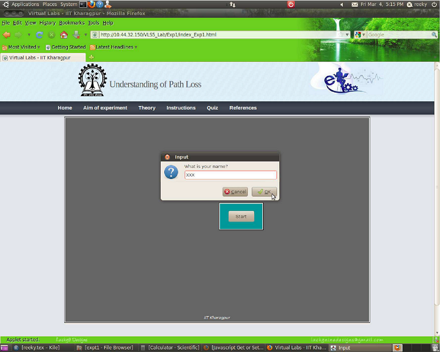
- Step 1:-Click on the START button.A page appears with a dialogue box asking for your name.Enter your name and click OK.
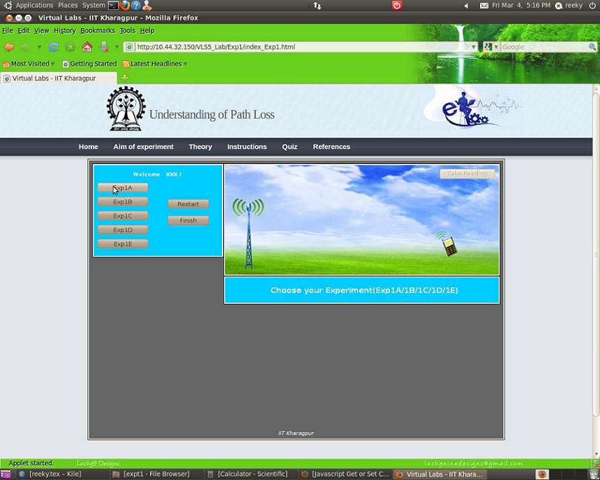
- Step 2:-Now the page appears where you can perform experiment1.There are 5 buttons(Exp1A Exp1B Exp1C Exp1D Exp1E) for five experiments to be performed . Choose which experiment you want to perform and click on any one of the button.
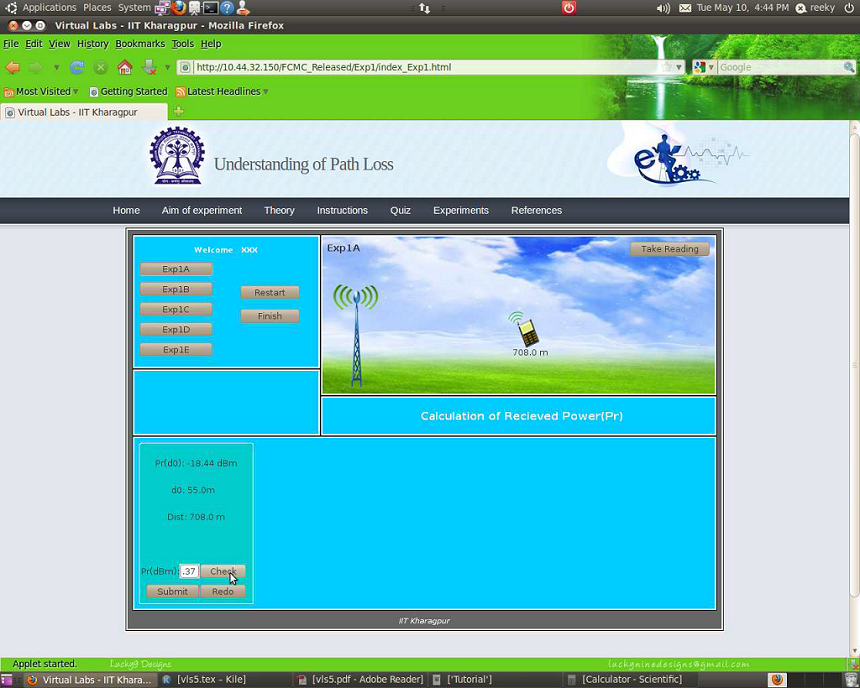
1.2 Performing Experiment 1A(Calculation of Received Power at a cer-tain Tx-Rx separation distance) :-
- Step 3:- Drag the mobile by placing the cursor on it and place it at a certain distance from the base station tower.
- Step 4:-Click on the button TAKE READING.Your input value get displayed.
- Step 5:-Now,calculate the value of the unknown parameter (for e.g.`P_r(d)`) manually by using the formulas given in the theory section. For example:- Given `P_r(d_0)=18.44dB`, Tx and Rx separation distance(d)= 708 m, `d_0=55 m`. So,using this formula `P_r(d)=P_r(d_0)+20log(d_0//d)` you can find the value of `P_r(d),P_r(d)=-18.44+20 log_10(55//708)=-40.37dBm.` Similarly,with the help of the formulas given in the theory section for expt1b,expt1c,expt1d and expt1e you can find the value of the unknown parameter for each of these experiments.
- Step 6:-Now,enter your manually calculated value of the unknown parameter in the box provided in the page.
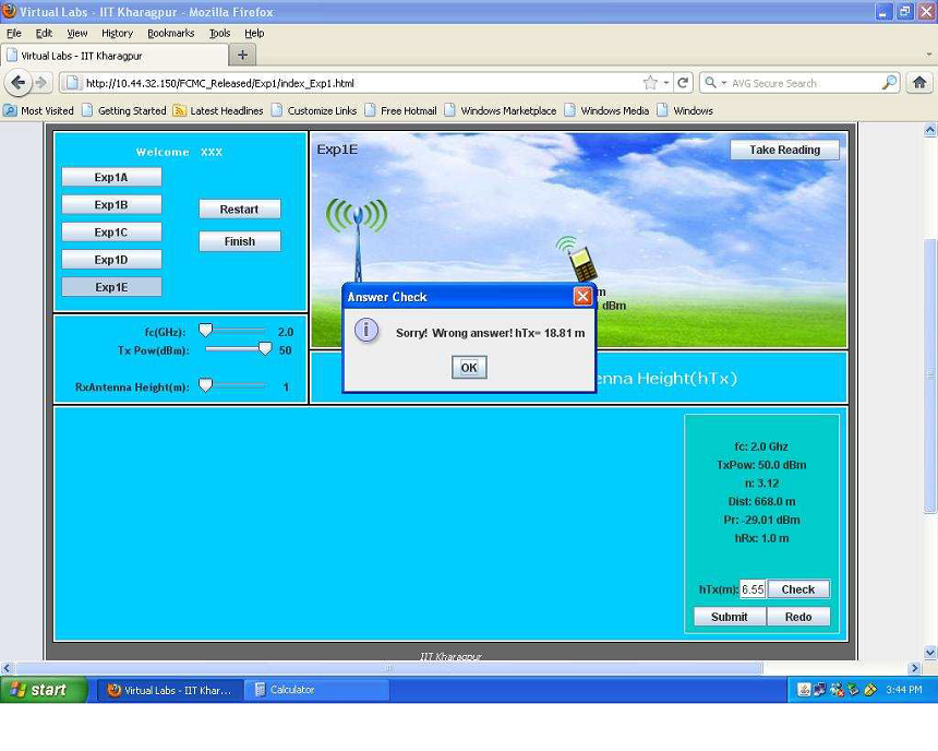
- Step 7:-Click on the button CHECK to verify whether your manually calculated value matches with the computed value of the unknown parameter.
- Step 8:-If your manually calculated value of the unknown parameter doesn't match with the com-puted value of the unknown parameter then a message box will appear with the message that your calculated value is wrong and it will return the exact value of the unknown parameter.If your cal-culated value of the unknown parameter is same as the computed value of the unknown parameter then the message box will let you know that your result is correct.
- Step 9:-Now, click on the button SUBMIT to submit your results
- Step 10:-You can redo the experiment by clicking on the button REDO.


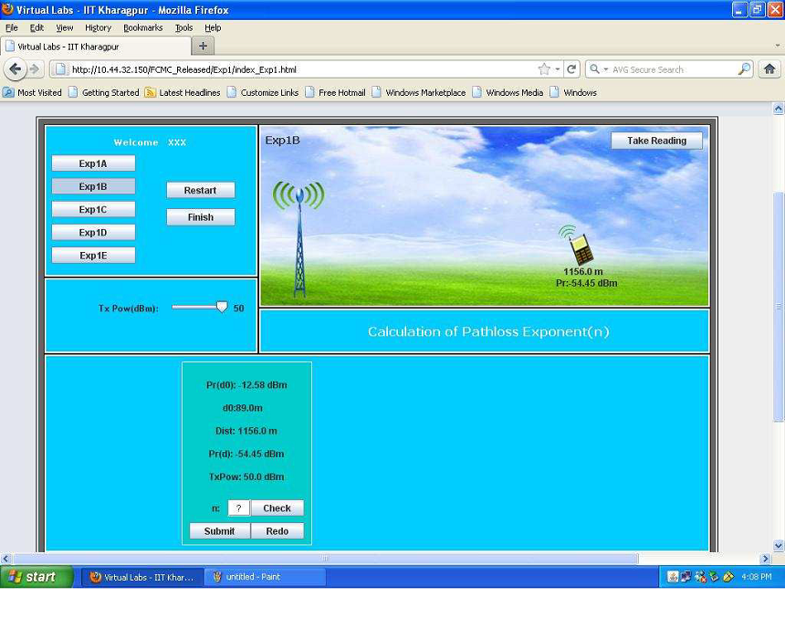
1.3 Performing Experiment 1B(Calculating the path loss exponent) :-
Follow the steps given below to perform Expt 1B
- Step 1:-Follow Step 2 of Expt 1A and select Expt 1B to perform it.
- Step 2:-Follow Step 3-4 of Expt 1A to record the input parameters needed for calculating the value of `n_p`.You can adjust the slider to change the value of transmit power.
- Step 3:- Now,use this formula to calculate `n_p`. Input Parameters :- `P_t=50dBm,P_r(d)=-54.45dBm,` `P_r(d_0)=-12.58dBm, d=1156 meters, d_0=89 meters. PL(d)=PL(d_0)+10**n_p**log_10(d//d_0)=P_t(d)` `-P_r(d)=P_t(d_0)-P_r(d_0)+10**n_p**log_10(d//d_0),50 +54.45 = 50 +12.58+10**n_p**log_10(1156//89),n_p=` 3.76 .
- Step 4:- Follow Steps 6-11 of Expt 1A to submit the results of Expt 1B.
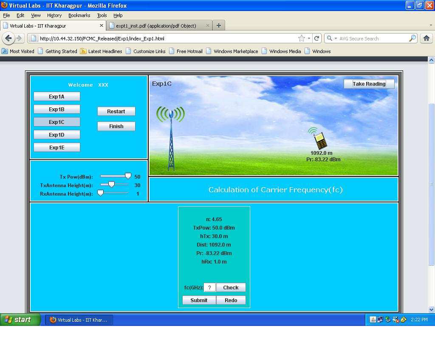
1.4 Performing Experiment 1C(Calculating fc) :-
Follow the steps given below to perform Expt1C
- Step 1:-Follow Step 2 of Expt 1A and select Expt 1C to perform it.
- Step 2:-Follow Step 3-4 of Expt 1A to record the input parameters needed for calculating the value of `f_c`.You can change the values of transmit power,transmit antenna height,receive antenna height by adjusting the sliders.
- Step 3:- Given `h_(BS)=30m,h_(UT)=1m,d=1092 m,n_p=4.65,P_t=50dBm,P_r(d)=-83.22dBm,`. Now, calculate PL(d) using the formula:-PL(d) = `P_t-P_r(d)=`50 - (-83.22) = 133.22 dBm. Now, use this formula to calculate `f_c`.PL(d) = `10n_plog_10(d)+7.8-18log_10(h_(tx))-18log_10(h_(rx))+20log_10(f_c)`. Putting the values, 133.22 = `10**4.65**log_10(1092)+7.8-18log_10(30)-18log_10(1)+20log_10(f_c)`. So,`f_c` = 3.44 GHz.
- Step 4:- Follow Steps 6-11 of Expt 1A to submit the results of Expt 1C.
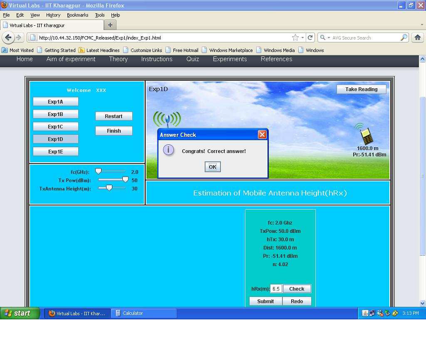
1.5 Performing Experiment 1D(Calculating `h_(UT)` ):-
Follow the steps given below to perform Expt1D
- Step 1:-Follow Step 2 of Expt 1A and select Expt 1D to perform it.
- Step 2:-Follow Step 3-4 of Expt 1A to record the input parameters needed for calculating the value of `h_(UT)` .You can change the values of transmit power,frequency,transmit antenna height by adjusting the sliders.
- Step 3:- Given `h_(BS)=30m,f_c=2GHz,d=1600m,n_p=4.02,P_t=50dBm,P_r(d)=-51.41dBm,`. Now, calculate PL(d) using the formula:-PL(d) = `P_t-P_r(d)=`50 -(-51.41) = 101.41 dBm. Now, use this formula to calculate `h_(rx)`.PL(d) = `10n_plog_10(d)+7.8-18log_10(h_(tx))-18log_10(h_(rx))+20log_10(f_c)`. Putting the values, 101.41 = `10**4.02**log_10(1600)+7.8-18log_10(30)-18log_10(h_(rx))+20log_10(2)`. So,`h_(rx)` = 6.5 meters.
- Step 4:- Follow Steps 6-11 of Expt 1A to submit the results of Expt 1D .

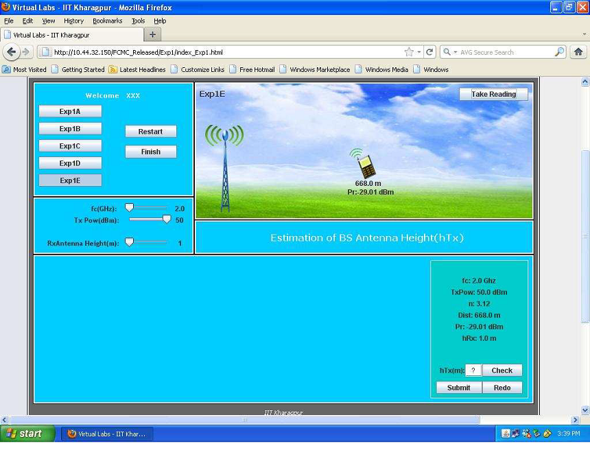
1.6 Performing Experiment 1E(Calculating `h_(BS)`) :-
Follow the steps given below to perform Expt1E
- Step 1:-Follow Step 2 of Expt 1A and select Expt 1E to perform it.
- Step 2:-Follow Step 3-4 of Expt 1A to record the input parameters needed for calculating the value of `h_(BS)`. You can change the values of transmit power,receive antenna height,frequency by adjusting the sliders.
- Step 3:- Given `h_(rx)=1m,f_c=2GHz,d=668m,n_p=3.12,P_t=50dBm,P_r(d)=-29.01dBm,`. Now, calculate PL(d) using the formula:-PL(d) = `P_t-P_r(d)=`50 -(-29.01) = 79.01 dBm. Now, use this formula to calculate `h_(BS)`.PL(d) = `10n_plog_10(d)+7.8-18log_10(h_(tx))-18log_10(1)+20log_10(f_c)`. Putting the values, 79.01= `10**3.12**log_10(668)+7.8-18log_10(h_(tx))-18log_10(h_(rx))+20log_10(2)`. So,`h_(tx)` = 16.55 meters.
- Step 4:- Follow Steps 6-11 of Expt 1A to submit the results of Expt 1E.
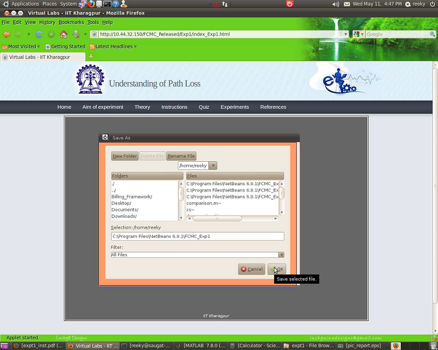
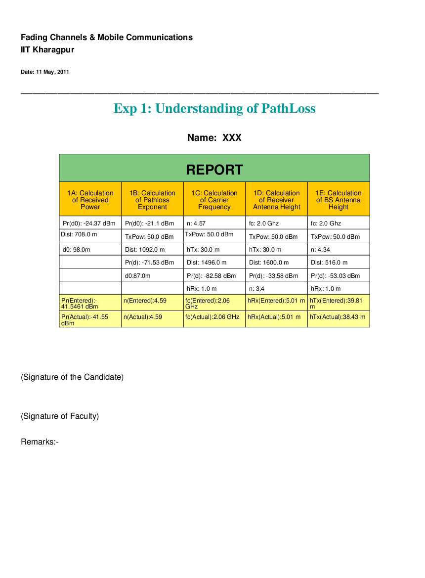
1.7 Generating and saving the Report :-
- Step 11:Click on the GENERATE REPORT button once you finish do ing all the experiments from Expt 1A to Expt 1E.
- Step 12:Click on the button SAVE to save your report.
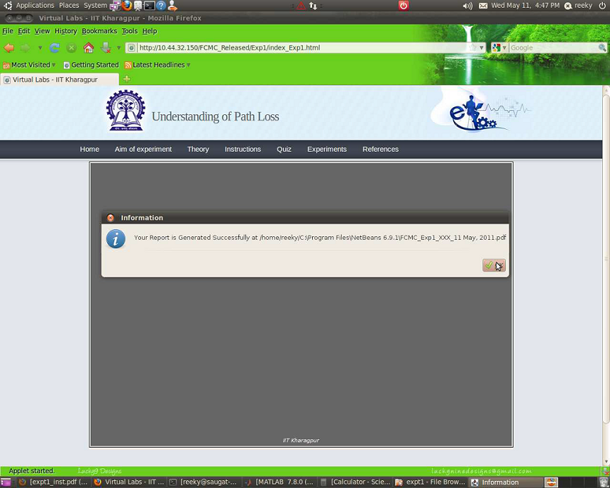
- Step 13:Finally, a message will appear that your report has been generated successfully.After viewing the message click on the OK button.
- Step 14:You can view the pdf report of the experiment you have done.


Test Your Knowledge!!

Books:
- Theodore S. Rappaport, 'Wireless Communications: Principles and Practice', 2nd Edition, Prentice Hall Communications Engineering and Emerging Technologies Series.
- Gordon L. Stuber, 'Principles of Mobile Communications', 2nd Edition, Gordon L. Stuber, Georgia Institute of Technology, Atlanta, Georgia, USA, Kluwer Academic Publishers.
- Report ITU-R, M.2135 - 'Guidelines for evaluation of radio interface technologies for IMTadvanced'.
NPTEL(National Programme on Technology Enhanced Learning):