Theory
The first step in the analysis of control system is to derive the mathematical model of the complete system. This would help in understanding the working of the complete system.
The Plant (Oven)
The plant to be controlled is an electric oven, the temperature of which must adjust itself in accordance with the reference or command. This is a thermal system which basically involves
transfer of heat from one section to another. In present case we are interested in transfer of heat from heater coil to the oven and leakage of heat from the oven to the atmosphere.
Here, a lumped parameter model is considered. For precise analysis, a distributed parameter model must be used. Another difficulty associated with temperature control system is that
the temperature rise is produced by energy input, which is controllable but the temperature fall is due to heat loss, which is uncontrollable. There are three modes of heat transfer
viz. conduction, convection, radiation. Heat transfer through radiation may be neglected in the present case since the temperatures involved are quite small.
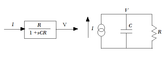 Fig. 1. Electrical Analogy
 Fig. 2. Closed loop Temperature Control System
For conductive and convective heat transfer,
$$ {\Theta = \alpha \Delta T} \tag{1}$$
where,
Θ = Rate of heat flow in Joule/sec.
Δ
T = Temperature difference in °C
α = Constant
Under assumption of linearity, the themal resistance is defined as,
$$R = \frac{ Temperature \ difference \ }{rate \ of \ heat \ flow}$$
$$ = \frac{\Delta T}{\Theta} = \frac{1}{\alpha} $$.
This is analogous to electrical resistance defined by
I = V/R. In a similar manner thermal capacitance of the mass is defined by
$$ \Theta = C \ \frac{d(\Delta T)}{dT} \tag{2}$$
which is analogous to the
V - I relationship of a capacitor, namely
I = C dV/dt. In the case of heat,
C = Rate of heat flow / Rate of temperature change.
The equation of an oven may now be written by combining the equations 1-2, implying
that a part of the heat input is used in increasing the temperature of the oven and the rest goes
out as loss. Thus
$$ \Theta = C \ \frac{dT}{dt} + \frac{1}{R} \ T, \tag{3}$$
with the initial condition
T (t = 0) = Tamb. Now, taking Laplace transform with zero
initial condition,
$$ \frac{T(s)}{\Theta(s)} = \frac{R}{1+sCR} \tag{4}$$
An analogous electrical network and block diagram may be drawn as shown in fig-1, defined
by the equation
$$I = C \frac{dV}{dt} + \frac{V}{R} \tag{5}$$
The temperature rise in response to the heat input is not instantaneous. A certain amount
of time is needed to transfer the heat by convection and conduction inside the oven. This requires a delay or transportation lag term,
e-sT2, to be included in the transfer
function, where
T2 is the time lag in seconds.
The open loop transfer function of the plant is given by
$$ G(s)= \frac{ke^{-sT_2}}{1+sT_1} \tag{6}$$
where
k = DC gain of the system,
T1 = Time Constant ,
T2 = Delay Time
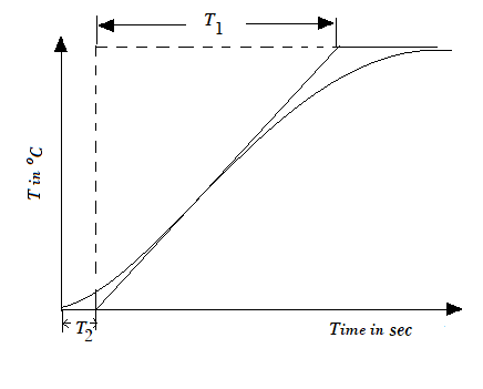 Fig. 3. Open loop response of the oven
Controller
Basic control actions commonly used in temperature control systems are,
1) Proportional
2) Proportional-Integral
3) Proportional-Integral-Derivative
4) ON-OFF or relay
These are described below.
Proportional Controller
Proportional controller is simply an amplifier of gain
kp which amplifies the error signal and passes it to the actuator.
A typical proportional controller may have input output characteristics as shown in Fig. 4.
Such controller gives a non-zero steady state error to step input for a type-0 system. The proportional block in the system consists of a
variable gain amplifier having a maximum value,
kp max of 20.
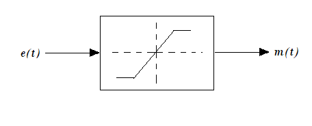 Fig. 4. P Controller
Proportional Integral Controller
Mathematical equation of such a controller is given by,
$$ m(t)= k_{p} e(t)+ k_i \int_{0}^{t}e(t)dt = k_p e(t)+\frac{1}{T_i}\int_{0}^{t}e(t)dt \tag{7}$$
It may be easily seen that this controller introduces a pole to origin, i.e. increases the system type by unity. The steady state error therefore gets reduced.
A block diagram representation is shown in fig 5. Qualitatively,
any small error signal
e(t), present in the system, would get continuously
integrated and generate actuator signal
m(t) forcing the plant output to exactly correspond to the reference input so that error is zero. In practical system the
error may not be zero due to imperfections in an electronic integrator caused by biased current needed, noise ,drift present and leakage of the integrator
capacitor. The integral block in the present system is realized with a circuit, that has a transfer function
$$ G_{r}(s)=\frac{1}{41 \ s}=\frac{k_{i}}{s} \tag{8}$$
The integral gain is therefore adjustable in the range 0 to 0.024 (approx).
 Fig. 5. PI Controller
Proportional Integral Derivative Controller
The governing equation here is,
$$ m(t)= k_{p} e(t)+ k_i \int_{0}^{t}e(t)dt + k_D\frac{de(t)}{dt} = k_p e(t)+\frac{1}{T_i}\int_{0}^{t}e(t)dt + T_D\frac{de(t)}{dt} \tag{9}$$
In laplace transform domain,
$$ \frac{M(s)}{E(s)}=(k_p + \frac{1}{T_i \ s} + T_D \ s) \tag{10}$$
A simple analysis would show that the derivative block essentially increases the damping ratio of the system and therefore improves the dynamic performance
by reducing the overshoot. The PID controller therefore helps in reducing the steady state error with an improvement in the transient response.
The derivative block in the present system is realized with a circuit, that has a transfer function
$$ G_{D}(s)=19.97 \ s \ (approx) \tag{11}$$
The derivative gain is therefore adjustable in the range of 0 to 20 approximately.
PID controller is one of the most widely used controller because of its simplicity. By adjusting its coefficients
kp, ki, kD
the controller can be used in variety of systems. The process of setting the controller coefficients to suit a given plant is known as tuning. There are many methods
of tuning a PID controller. In present experiment, the method of Ziegler-Nichol has been introduced which is suitable for the oven Control System.
According to the Ziegler-Nichol rule,
in P control,
$$ k_p = (\frac{1}{k})\frac{T_1}{T_2} \tag{12}$$
in PI control,
$$ k_p = (\frac{0.9}{k})\frac{T_1}{T_2} \tag{13}$$
$$ k_i = \frac{1}{3.3T_2} \tag{14}$$
in PID control,
$$ k_p = (\frac{1.2}{k})\frac{T_1}{T_2} \tag{15}$$
$$ k_i = \frac{1}{2T_2} \tag{16}$$
$$ k_D = 0.5T_2 \tag{17}$$
P-control potentiometer setting:
Calculate the value of
kp for each type of control using the Ziegler-Nichol rule. The formula for
kp is for an unity feedback system and has the
dimension of Volts/°C. In the present unit a temperature sensor having sensitivity of 10mV/°C (0.01 V/°C) is used between oven output and controller input. Hence, divide the
kp calculated above by 0.01 and then
by the
kp max value (20) to get the potentiometer setting.
I-control potentiometer setting:
Calculate the value of
ki for each type of control using the Ziegler-Nichol rule. Then divide that calculated value by
ki max value (0.024) to get the potentiometer setting.
D-control potentiometer setting:
Calculate the value of
kD for each type of control using the Ziegler-Nichol rule. Then divide that calculated value by
kD max value (23.5) to get the potentiometer setting.
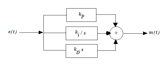 Fig. 6. PID Controller
ON-OFF or Relay type controllers :
It is also reffered to as two position controllers, consist of a simple and inexpensive switch/relay and are, therefore, used very commonly in both industrial and domestic control systems.
Typical applications include air-conditioner and refrigerators, ovens, heaters with thermostat. Solenoid operated two position valves are commonly used in hydraulic and pneumatic systems.
The basic input-output behaviour of this controller is shown in Fig. 7. The two positions of the controller are
M1 and
M2, and
H is the hysteresis or differential gap.
The hysteresis is necessary, as it enables the controller output to remain at its present value till the input or error has increased a little beyond zero. Hysteresis helps in avoiding too frequent
switching of the controller, although a large value results in greater errors. The response of the system with ON-OFF controller is shown in Fig. 8. Describing function technique is a standard method
for the analysis of non-linear systems, for instance, one with an ON-OFF controller.
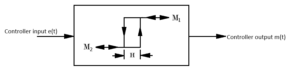 Fig. 7. ON-OFF Controller
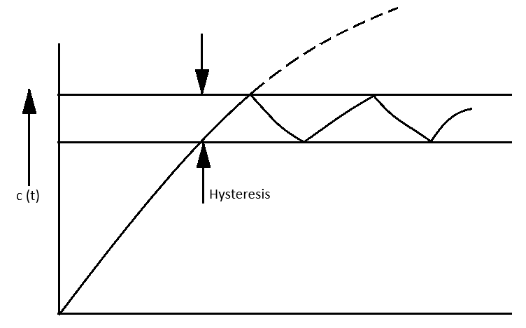 Fig. 8. Response of ON-OFF control system