|| DESIGN OF LOW PASS FILTER USING FDATOOL:||

 

| STEPS TO DESIGN FILTER USING FDATOOL |

 

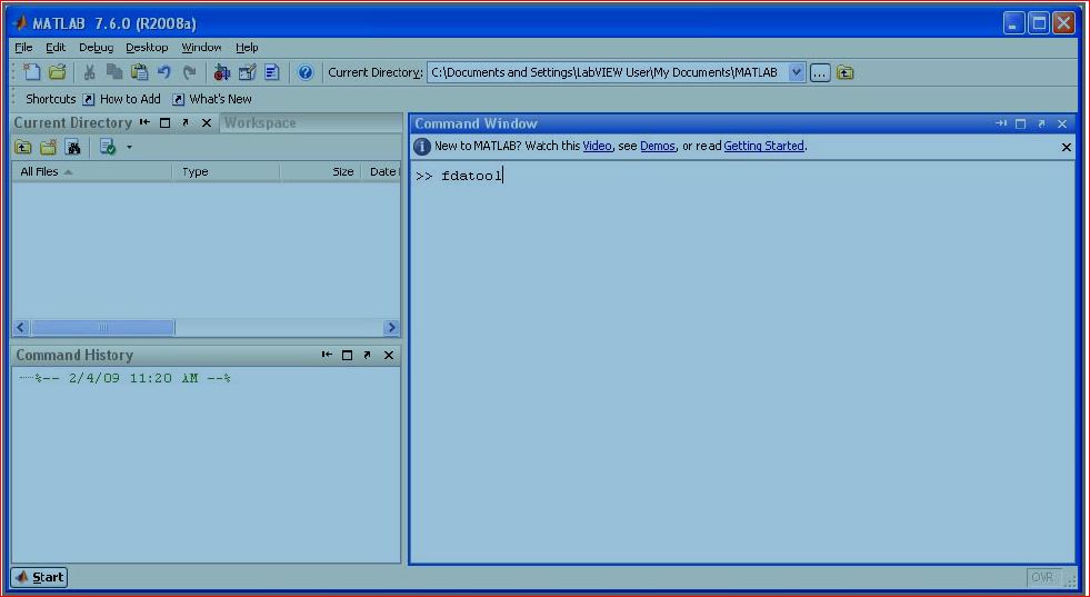
Open up MATLAB and type FDATOOL into the workspace and hit Enter.

 

 

• This GUI allows us to design many different types of digital filters very easily. We can specify the type of filter and the design type, as well as the pass and stop band frequencies. In addition, we can specify the attenuation in the pass and stop band to give us the desired filter response (by changing the values on the bottom right corner of the window). On clicking the "Design Filter" button, fdatool automatically designs a filter of the lowest order, which achieves these attenuations. We can also specify the order.

• Select "Lowpass" and "Equiripple" as response type and design method respectively from bottom left, as shown in the figure.

 

 

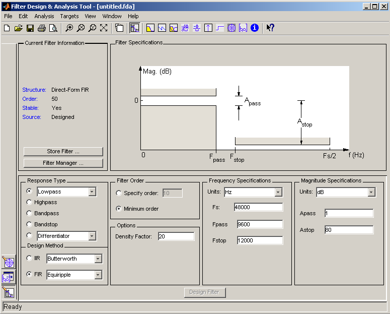
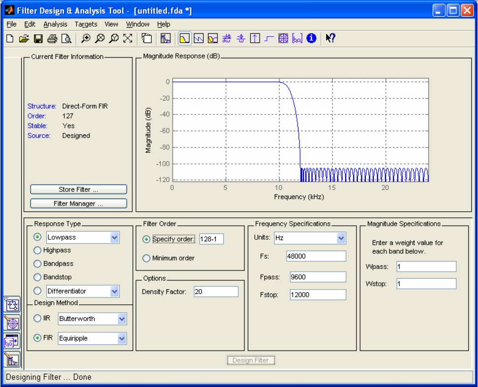
• Specify the order of the filter, the sampling frequency of the system for which the filter is to be used, the upper frequency (where the pass band ends), and the stop frequency (where the stop band starts). It may be useful to specify the order as N-1, where N is the number of coefficients that the filter will have. For 128-1=127 order filter have 128 coefficients. In this tutorial, Sampling Frequency Fs is chosen as, Fs = 48000 Hz, Pass band frequency is Fpass = 9600 Hz, and stop band frequency is Fstop = 12000 Hz. Select the passband and stopband weights. If both the bands are equal the weights should be equal. If the passband is narrow then a higher weight has to be used here to ensure matching of the resulting response.

 

 

• Hit the "Design filter" button to get the filter. As seen in the figure below, the filter has been generated and the response has been plotted.

 

 

CHANGING ANALYSIS PARAMETERS:

 

• By right clicking on the plot and selecting Analysis parameters, we can display a dialog box for changing analysis specific parameters.

 

 

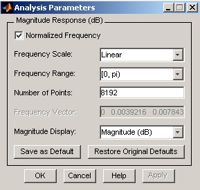
• To save the displayed parameters as the default values, click Save as Default. To restore the MATLAB-defined default values, click Restore Original Defaults.

 

Exporting The Filter:

 

• Once you are satisfied with your design, you can export your filter to the following destinations:

 

MATLAB workspace
MAT-file
Text-file
Select Export from the File menu.

 

 

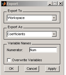
• If exporting to the MATLAB workspace, you can export as coefficients or as an object by selecting from the Export from the pulldown menu.

 

SIMULATION USING MATLAB CODE:

 

This experiment requires MATLAB with Signal Processing toolbox. The fdatool can be used as given in the video tab. For the simulation the student needs to write a program which uses filter function and simulate in the MATLAB. The student version of MATLAB is available here.

The following program is used to simulate a filter which has the design specifications as follows

1. Low Pass FIR filter
2. Order =5
3. Sampling frequency 2000 Hz (2kHz)
4. Passband upto 400Hz
5. Tranisition Band 400Hz-500Hz
6. Design Method in fdatool is least square
7. Weights for errors in the passband=2 and stopband=1
8. coefficients saved as h in the filt.mat file
9. Tested using the following program

   

Open a new m file and copy-paste the following code.

 

clear all  % clears all variables from the workspace
close all %closes all windows
clc % clears the screen

load filt  % loads filter coefficients stored in filt.mat as variable h

% generate unity amplitude 0 phase sine wave of 1000 samples of variable frequency in the loop
n=[1:1000]';
Fs=2000; % Sampling frequency
Ts=1/Fs;%sampling time
for f=1:10:900
   
x=sin(2*pi*f*n*Ts);

% filter the signal x

% the output y is intialized to 0 for N-1 consecutive samples = order of the
% filter
N=length(h);

y=zeros(N-1,1);

for k=N:length(x)
        y(k)=0;
    for m=1:N  % N+1= no of filter coefficients
    y(k)=y(k)+h(N-m+1)*x(k-m+1);
    end
end
subplot(211)
plot(y(200:300))
title(f) % shows the frequency at which the plot is shown
ylim([-1.5 1.5]);
shg
subplot(212)
plot([x(200:300) y(200:300)])
title('relative phase')
pause
end

 

 

Save the m file and simulate.