
The objective of time-frequency analysis is to decompose energy of a signal in both time and frequency. This decomposition helps to operate the signal in a controlled way and to construct signal with the specific properties. The basic tool to implement this decomposition is the Classical Fourier transform. Classical Fourier Transform are generally most suitable for the time-stationary signals. For the signals that evolve in time, we can use:
- Linear time-frequency representations (such as short-time Fourier transforms, wavelet transforms etc.)
- Quadratic time-frequency representations (for instance Cohen's class, including the Wigner distribution originating from quantum mechanics)
Need for Time-Frequency analysis
The two classical representation of a signal are the time-domain `s(t)` and frequency domain `s(f)` representation. In both the representations, the variables `t` and `f` are treated as mutually exclusive. Hence in order to obtain a representation in terms of one variable, the other one should be integrated out. The frequency representation is essentially averaged over the values of the time representation at all times, and the time representation is essentially averaged over the values of the frequency representation at all frequencies. In the time frequency distribution the variable `t` and `f` are not mutually exclusive, but are present together. The time frequency distribution is localized in `t` and `f`.
Characteristics of time frequency representation
The use of time-frequency distribution is based on particular?s assumption concerning the properties of the Time-Frequency distribution. The following characteristics illustrate uses of time-frequency distribution.
- The raw signal can be analyzed in the time-frequency (`t,f`) domain to identify its characteristics such as frequency variation, time variation, number of components, relative amplitudes, etc.
- The component can be separated from each other as well as from background noise by filtering in time frequency (`t,f`) domain .
- Synthesize the filtered time-frequency representation in time domain.
- Specific components can be analyzed separately such as tracking of instantaneous amplitude, instantaneous frequency, instantaneous bandwidth, etc.
- A mathematical model of a signal can be chosen which clearly shows the significant characteristics, such as IF.

Time Frequency Analysis
Fourier transform is a common method for signal analysis. Fourier transform only focuses on frequency domain signal analysis. It cannot analyze the variations of frequency with respect to time.
Time frequency analysis deals with the spectrum utilization of non stationary signals such as speed, audio etc. Short Time Fourier Transform (STFT) is the simplest two dimensional time frequency representation created by computing the Fourier transform and using a sliding temporal window.
Short Time Fourier Transform(STFT)
By using Short Time Fourier transform (STFT) we can observe the changes in frequency with respect to time. The magnitude of STFT is called as spectrogram.
The Short Time Fourier transform (STFT) of signal `x(t)` using a window function `g(t)` is defined as.
`STFT(f,s) = int_-oo^oo x(t)g(t-s)e^(-2pif_tj)dt`
Continuous-time STFT
In continuous-time STFT, the function to be transformed is multiplied by a window function which is nonzero for only a short period of time. The Fourier transform (a one-dimensional function) of the resulting signal is taken as the window is slid along the time axis, resulting in a two-dimensional representation of the signal. Mathematically, this is written as:
`STFT{x(t)}(tau,omega) = X(tau,omega) = int_-oo^oo x(t)w(t-tau)e^(-jomegat)dt`
Where `w(t)` is the window function, commonly a Hann window or Gaussian bell centered around zero, and `x(t)` is the signal to be transformed. `X(tau,omega)` is essentially the Fourier Transform of `x(t)w(t-tau)`, a complex function representing the phase and magnitude of the signal over time and frequency.
Discrete-time STFT
In discrete time STFT, the data to be transformed could be broken up into chunks or frames (which usually overlap each other, to reduce artifacts at the boundary). Each chunk is Fourier transformed, and the complex result is added to a matrix, which records magnitude and phase for each point in time and frequency. This can be expressed as:
`STFT{x[n]}(m,omega) = X(m,omega) = sum_(n=-oo)^oo x[n]w[n-m]e^(-jomegan)`
Likewise, with signal `x[n]` and window `w[n]`. In this case, m is discrete and `omega` is continuous, but in most typical applications the STFT is performed on a computer using the Fast Fourier Transform, so both variables are discrete and quantized.

The objective of this experiment is to perform time-frequency analysis of stationary and non-stationary signals. Some of these signals are actual signals acquired from operating machine and equipment.

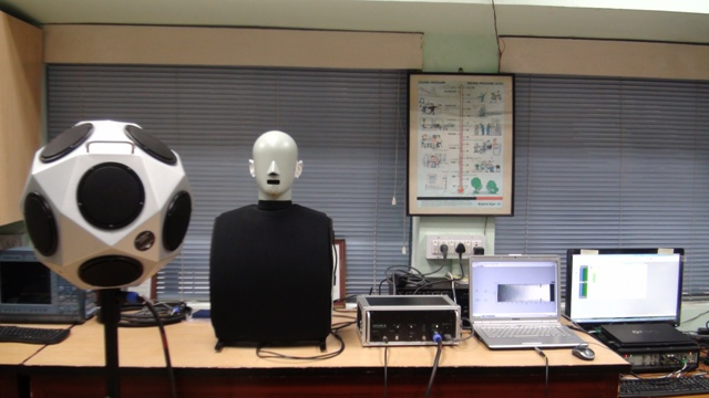
Head and Torso Simulator (HATS)
Head and Torso Simulator is a mannequin with built-in ear and mouth simulators that provides a realistic reproduction of the acoustic properties of an average adult human head and torso. It is ideal for performance in-situ electro acoustic tests on:
- Telephone handsets (including mobile and cordless)
- Headsets
- Audio conference devices
- Microphones
- Headphones
- Hearing aids
- Hearing protectors
Omni Power Sound Source
For most building acoustics measurements, the sound source must radiate sound evenly in all directions to give reproducible and reliable results; therefore, the relevant building acoustics measurements standards (ISO 140 and ISO3382) require the use of an unidirectional sound source.
Omni Power Omni directional Sound Source Type 4292-L uses a cluster of 12 loudspeakers in a dodecahedral configuration that radiates sound evenly with a spherical distribution. All 12 speakers are connected in a series-parallel network to ensure both in-phase operation and an impedance that matches the power amplifier. The entire assembly weighs no more than 8 kg and is fitted with a convenient lifting handle that does not measurably interfere with the sound field.
Creating and Playing Stationary and Non-stationary Sounds
Note: Before going to download required application, Installer should be downloaded. After downloading this installer, extract the files. Click on the setup icon is located on the volume folder of this attachment. The downloadable attachament is given in following attachament. In case of LabVIEW 8.5 was pre-installed, please eliminate this step.
Note: After installing the setup, please download and install the application.exe file which is given in following attachment.
.png)
Note: To create stationary sound wave the starting and the end frequency should be kept same.

Time frequency analysis of stationary and non stationary sounds have been done for analysing the variations of frequency with respect to time.
Time Frequency Analysis of Stationary Sound Waves
1. A time frequency analysis of sine wave at 1000 Hz frequency
Time frequency plot of sine wave at 1000 Hz frequency
.png)
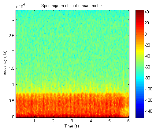
2. A time frequency analysis of boat stream motor
Click the button to hear the sound file of boat stream motor
Time frequency plot of boat stream motor
Time Frequency Analysis of Non-stationary Sound Waves
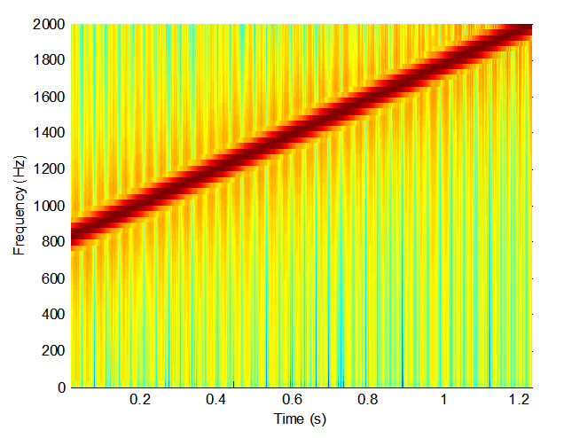
1. A time frequency analysis of sweep sound between 800-2000Hz frequency
Time frequency plot of sweep sound between 800-2000Hz frequency
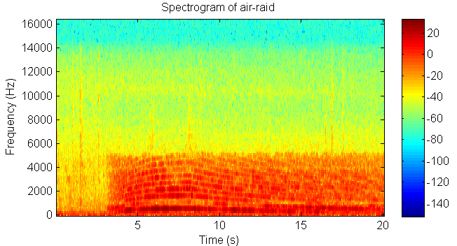
2. A time frequency analysis of air-raid
Click the button to hear the sound file of air-raid
Time frequency plot of air raid
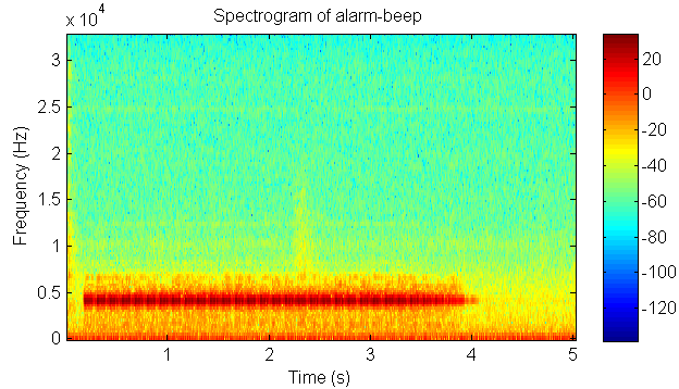
3. A time frequency analysis of alarm beep
Click the button to hear the sound file of alarm beep
Time frequency plot of alarm beep
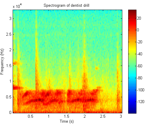
4. A time frequency analysis of dentist drill
Click the button to hear the sound file of dentist drill
Time frequency plot of dentist drill
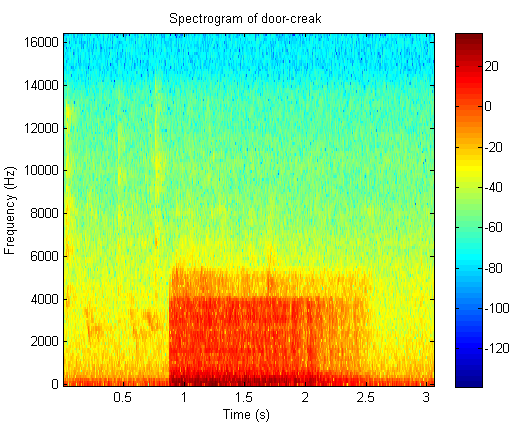
5. A time frequency analysis of door creak
Click the button to hear the sound file of door creak
Time frequency plot of door creak
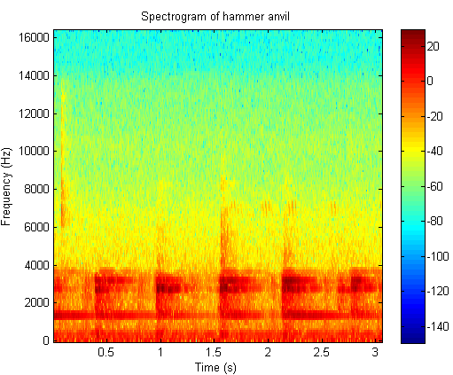
6. A time frequency analysis of hammer anvil
Click the button to hear the sound file of hammer anvil
Time frequency plot of hammer anvil
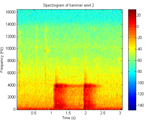
7. A time frequency analysis of hammer anvil2
Click the button to hear the sound file of hammer anvil2
Time frequency plot of hammer anvil2
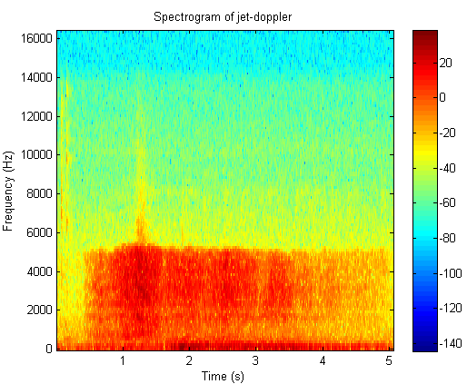
8. A time frequency analysis of jet doppler1
Click the button to hear the sound file of jet doppler1
Time frequency plot of jet doppler1
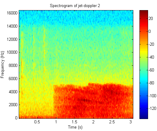
9. A time frequency analysis of jet doppler2
Click the button to hear the sound file of jet doppler2
Time frequency plot of jet doppler2
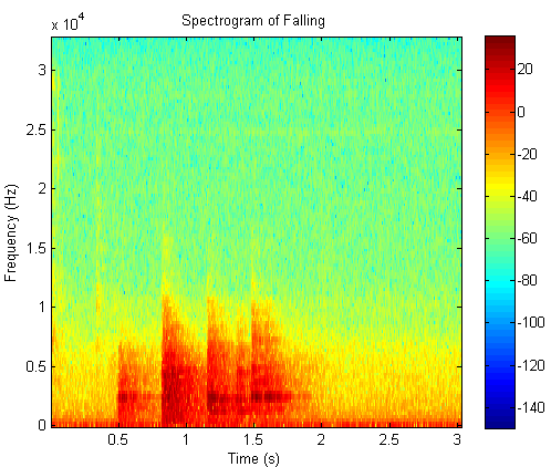
10. A time frequency analysis of falling object
Click the button to hear the sound file of falling object
Time frequency plot of falling object
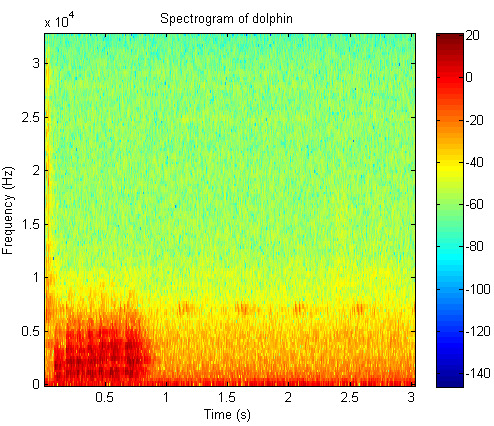
11. A time frequency analysis of dolphin whistle
Click the button to hear the sound file of dolphin whistle
Time frequency plot of dolphin whistle

Books
- Léon Cohen, "Time-Frequency Analysis," Prentice Hall PTR, 1995
- Robert W. Ramirez, "The FFT: Fundamental and Concepts," Prentice hall, Inc. Englewood Cliffs, N.J., 1985