
1. What is Signal?
To answer this question precisely is not a simple task. A signal is a function representing a physical quantity or variable, and typically it contains information about the behaviour or nature of the phenomenon. Everything from a smallest unit (cell) to complex unit (human) is the result of appropriate processing of time signals. Examples are human voices, chirping of birds, communication between bees through dance and gestures (sign language) etc. Some examples of modern high speed signals are radio frequency waves, variation of light intensity in optical fibres, sound waves produced at supersonic speed of airplanes. Thus, we are surrounded by endless variety of signals which may carry some sort of information from one place to another.

Fig. 1: Modern example - AM transmitter system

Fig. 2: Simplified oscilloscope operation
2. How can we observe these signals?
The traditional to observe is to view them in the time domain. The time domain is a record of what happened to a parameter of the system versus time. For instance, in a RC circuit the signal may represent the voltage across the capacitor or the current flowing in the resistor with sequences of time. There are lot of ways to record the variable which is to be measured with time. Figure 3 shows direct and indirect recording of displacement of mass of a simple spring mass system. The resulting graph is a record of the displacement of the mass versus time, a time domain view of displacement.
 Direct and (b) Indirect representation of displacement in time domain")
Fig. 3: (a) Direct and (b) Indirect representation of displacement in time domain
3. Why do we need to know about the signal?
Signals convey information between the measurement station and the observer. The information in the signal obtained after processing the signal provides information about the state of the measurement station. In other words by signal processing one is able to know about the state of a system. Depending upon the state of the system, necessary actions can be initiated, like in controlling the system, know the condition of the system etc. Thus signal processing has a very important role to play in providing information about a mechanical system. The signal as measured by a transducer connected on the mechanical system is usually analog in nature as shown in Fig 4.

Fig 4: An analog signal produced by a microphone in response to a continuously changing sound
Analog signals are continuous in time. Any information may be conveyed by these signals; often such a signal is a measured response to changes in physical phenomena, such as sound, light, temperature, position, or pressure, and is achieved using a transducer. These analog signals can also be processed by electronics hardware to extract the features in the signal like its, mean, power, maximum, minimum value etc. However analog processing of the signals is limited by the electronics hardware available. Alternately if the analog signals can be converted into digital signals by a suitable analog to digital converter (A/D) converter, and the signal stored in a computer as digital numbers, there is practically no limit to the processing of these signals in the digital domain. Fig. 5 represents the conversion of analog signals to digital signals by data acquisition system.

Fig. 5: Conventional computerized signal acquisition system
Thus the advantage of digital signal processing, is that it is very economic and efficient manner in which signals can be processed to extract features and gain insight into the mechanical system producing such signals.
The basics of the signals such as fundamentals of the signals, types of signals, properties of the signals etc. are introduced in the theory section. Further, different modules based on the methods of the generation of the input signals are used to evaluate the features of the different signals. The detailed procedures of the modules are also presented in separate sections. These modules give enough information to understand the nature and significance of the signals. Those who desire the more details, references are listed.

1. How can we represent signals?
Mathematically, a signal, usually is represented as a function of an independent variable time, `t`. Thus, a signal is denoted by `x(t)`. A sinusoidal signal obtained from oscilloscope can be represent in following form
`x(t) = x_maxsin(omegat + phi)`
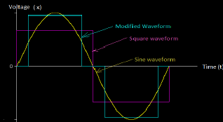
Fig.: Representation of different signals obtained from oscilloscope
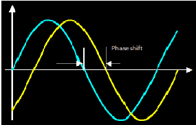
To represent a sinusoidal signal we require three parameters that are maximum amplitude , angular frequency and phase. Frequency (`f`) represent the how often signal goes through repeated cycles, i.e. `omega = 2pif`. For example if the signal repeats in `T` (time period) second then the frequency (in Hz) will be
`f = 1/T`
Phase is a fraction of cycle which is elapsed from an arbitrary point. For example, has delayed by 1/4th of its cycle then it becomes
`x(t-1/4T) = Asin[2pif(t-1/4T)+phi]`
or, `x(t-1/4T) = Asin[2pift-pi/2+phi]`,
whose "phase" is now `(phi-pi/2)`. It has been shifted by `pi/2` radians.
2. How can we classify the signals?
The general classification of signals is classified into following categories
(a) Continuous-Time and Discrete-Time Signals:
A Signal `x(t)` is a Continuous-Time signal if it is a continuous variable. If `t` is a discrete variable, that is, `x(t)` is defined at discrete times, then `x(t)` is a discrete-time signal . Since a discrete-time signal is defined at discrete times, a discrete-time signal is often identified as a sequence of numbers, denoted by `x{n}` or `x[n]` where `n` = integer.
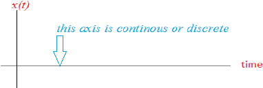
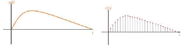
Fig.: Continuous signal (takes values in the set `[0,30]`) Discrete signal (takes values at the integers `{0,1,....,30}`)
(b) Analog and Digital Signals:
If a continuous-time signal `x(t)` can take on any value in the continuous interval `(a,b)`, where `a` may be `-oo` and `b` may be `+oo`, then the continuous-time signal `x(t)` is called an analog signal. If a discrete-time signal `x[n]` can be take on only a finite number of distinct values, then we call this a digital signal.

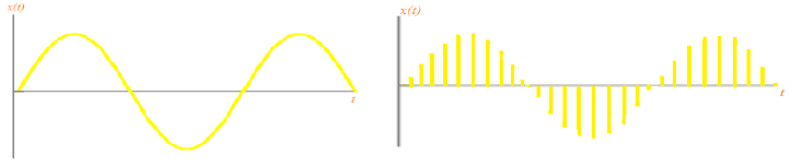
Fig.: (a) Analog and (b) Digital Signal
(c) Real and Complex Signals
A signal `x(t`) is a real signal if its value is a real number and a signal `x(t)` is a complex signal if its value is a complex number. A general complex signal `x(t)` is a function of the form
`x(t) = x_1(t) + jx_2(t)`
where `x_1(t)` and `x_2(t)` are real signals and `j=sqrt(-1)`.
Note that `t` represents either a continuous or a discrete variable.

Fig.: Complex Exponential Signal
(d) Deterministic and Random Signals
Deterministic signals are those signals whose values are completely specified from any given time, thus, can be modelled by a known function of time `t`. Random signals are those signals that take random values at any given time and must be characterized statistically.

Fig.: Deterministic Signal
Fig.: Random Signal
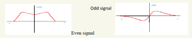
(e) Even and Odd Signals
A signal `x(t)` or `x[n]` is referred to as an even signal if
`x(-t) = x(t) , x[-n] = x[n]`
A signal `x(t)` or `x[n]` is referred to as an odd signal if
`x(-t) = -x(t) , x[-n] = -x[n]`
(f) Periodic and Non-periodic Signals
A continuous time signal `x(t)` is said to be periodic with time `T` if there is a positive non-zero value of `T` for which
`x(t + mT) = x(t)`
for all `t` and any integer `m`. The fundamental period `T_0` of `x(t)` is the smallest value of `T`.
Characteristics of signals


3. Criterion for the Signal
A more quantitative criterion is provided by the sampling theorem which states that for accurate representation of a signal `x(t)` by its time samples `x[n]`, two conditions must be met:
Signal sampling
To represent the signal in digital computers, we need to sample the signals. To sample signal `x(t)` must be bandlimited, that is, its frequency spectrum must be limited to contain frequencies upto some maximum frequency, say `f_max` and no frequencies beyond that.
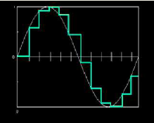
Sampling Rate: the rate at which the samples are digitized from the original signal is called sampling rate. Higher the sample rate, higher is the accuracy.

Sampling Theorem
The sampling rate `f_s` must be chosen to be at least twice the maximum frequency `f_max`, that is,
`f_s >= 2f_max`
or, in terms of the sampling interval
`T <= 1/(2f_max)`
4. What can you measure in Signals
There are lots of different measures in signals that you can measure. A few of them are
Arithmetic Mean:
The measurement mean is the mean value of all samples in the sample range.
Mean` = bar x = (1/N)sum_(i=m)^n x_i`
Maximum:
Maximum finds the highest point in a set of values in signals.
Range:
Range (maximum-minimum) finds the value of the range from the lowest point to the highest point in a set of values in signals.
Root Mean Square (RMS):
Root Mean square is also known as the quadratic mean, a statistical measure of the magnitude of a varying quantity. The measurement RMS is equal to the square root of mean of the squares of all samples in the sample range.
RMS` = sqrt((1/N)sum_(i=m)^n (x_i)^2)`
Variance:
The measurement variance is a measure of how values are distributed around the mean value.
Variance` = sigma^2 = (1/N)sum_(i=m)^n (x_i-bar x)^2`
Standard Deviation:
The measurement standard deviation (`sigma`) is equal to the square root of the variance. It is equal to the RMS value for signals with a zero mean value (AC signals).
`sigma = sqrt(Variance) = sqrt((1/N)sum_(i=m)^n (x_i-bar x)^2)`
Skewness:
Skewness is a measure of symmetry and is the normalized form of third-order moment about the mean. Skewness is indicated by the following formula:
Skewness` = (Third Moment)/sigma^3`
or, Skewness` = (sum_(i=m)^n (x_i-bar x)^3)/((N-1)sigma^3)`
Kurtosis:
Kurtosis is a measure of peakedness and is a normalized form of the fourth-order moment about mean. Kurtosis is indicated by the following formula:
Kurtosis` = (Fourth Moment)/sigma^4`
or, Kurtosis` = (sum_(i=m)^n (x_i-bar x)^4)/((N-1)sigma^4)`
Kurtosis of a signal is useful to detect the presence of an impulse within the signal.It is widely used for detecting discrete, impulsive faults in rolling element bearings. Good bearings tend to have a kurtosis value of approx. 3 and bearings with impulsive defects tend to have higher values (generally >6)
Crest Factor:
Crest Factor is the ratio of peak amplitude to RMS value of the signal. It is an important parameter which is used in measurement of intensity of bearing damage. As the damage increases, the waveform becomes far more impulsive, with higher peak values. So crest factor is sometimes called as the impact index. As a thumb rule, good bearings have vibration crestfactor of approx. 2.5-3.5 and damaged bearings have crest factor >3.5.
`C = (|x|_(peak))/(x_(rms))`
Form Factor:
Form Factor is the ratio of RMS value to the arithmetic mean of absolute values of all points of the signal.
`K_f = (x_(rms))/bar x`

Introduction to basics and fundamentals of signal analysis and signal feature extraction in time domain.

The experiment of basics of dynamic signals is divided into three modules based on method of signal generation. For each module the signal parameters are evaluated by using the LabView 8.5 software. One can understand and estimate these parameters for different type of signals and also observe the variation of these parameters with input parameters.
Types of signal generation used in this experiment are:
- By user defined waveforms
- By mathematical function
- By measured data
1. By user defined waveforms
The signals are generated for commonly used mathematical waveforms
In general, the user defined waveforms are:
(a) square wave
(b) sine wave
(c) triangular wave
(d) sawtooth wave
The signals are generated by providing the amplitude, frequency and offset and sampling rate.
2. By mathematical function
The signals are generated by providing mathematical expression for different waveform in string of characters. The advantage of this type of signal generation is we can generate any type of signals like random signal, ramp, or we can add two signals. etc.
3. By measured data
Signals can also generated by proving sampling to measured data which may be generated from real experiment.
Based on this experiment is categorized into three sub experiments:

Test Your Knowledge!!

1. Why do we need to know about signals?
2. What are the types of signals and how are they represented?
3. What is sinusoidal signals and how are they represented?
4. What are the parameters of given mathematical expression for the voltage signal as a function of time?
5. Consider the signal defined for all real `t` described by:
`f(t) = ((sin(2t)/t, > 1), (0, t < 1))`
Prove that the signal is continuous, analog, aperiodic, infinite length and deterministic.
6. How the sine wave can be mixed with DC signals, which is also known as complex waveform?

Books
- Robert W. Ramirez, "The FFT: Fundamental and Concepts," Prentice hall, Inc. Englewood Cliffs, N.J., 1985
Videos