
This experiment enables a student to learn
- Basics of IIR filter designing and its implimentation.
- Filter designing techniques like Butterworth, Chebyshev 1, Chebyshev 2, Elliptic etc.

Finite Impulse Response (FIR) Filter
IIR filters are digital filters with infinite impulse response. Unlike FIR filters, they have the feedback (a recursive part of a filter) and are known as recursive digital filters therefore. Block diagrams of FIR and IIR filters
For this reason IIR filters have much better frequency response than FIR filters of the same order. Unlike FIR filters, their phase characteristic is not linear which can cause a problem to the systems which need phase linearity. For this reason, it is not preferable to use IIR filters in digital signal processing when the phase is of the essence.
Otherwise, when the linear phase characteristic is not important, the use of IIR filters is an excellent solution.
There is one problem known as a potential instability that is typical of IIR filters only. FIR filters do not have such a problem as they do not have the feedback. For this reason, it is always necessary to check after the design process whether the resulting IIR filter is stable or not.
IIR filters can be designed using different methods. One of the most commonly used is via the reference analog prototype filter. This method is the best for designing all standard types of filters such as low-pass, high-pass, band-pass and band-stop filters.
Figure 10.1 illustrates the block diagram of this method.

Fig-10.1
FIR filters can have linear phase characteristic, which is not typical of IIR filters. When it is necessary to have linear phase characteristic,
FIR filters are the only available solution. In other cases when linear phase characteristic is not necessary, such as speech signal processing,
FIR filters are not good solution. IIR filters should be used instead. The resulting filter order is considerably lower for the same frequency response.
The filter order determines the number of filter delay lines, i.e. number of input and output samples that should be saved in order that the next output sample can be computed. For instance, if the filter order is 10, it means that it is necessary to save 10 input samples plus 10 output samples preceeding the current sample. All these 21 samples will affect the next output sample.
The IIR filter transfer function is a ratio of two polynomials of complex variable z-1. The numerator defines location of zeros, whereas the denominator defines location of poles of the resulting IIR filter transfer function.
Figure 10.2. illustrates input and output signals of the system with non-linear phase characteristic.

Fig-10.2
The system introduces phase shift of 0 radians at frequency of ω and Π radians at three times higher frequency. Input signal consists of nature frequency ω and harmonics with the same amplitude at three times higher frequency. Figure on the left illustrates an input signal, whereas Figure on the right illustrates an output signal. As seen, these two signals have different waveforms. Neither the power of the signal nor amplitudes of particular harmonics have been changed, but the phase of the second harmonic.
Assume that an input represents a speech signal where the phase is not important. In this case such phase distorsion would be negligable as the system satisfies the stated requirements. Otherwise, if the phase is important, such a huge distorsion mustn’t be allowed.
Infinite impulse response (IIR) filter design
The most commonly used IIR filter design method uses reference analog prototype filter. It is the best method to use when designing standard filters such as low-pass, high-pass, bandpass and band-stop filters
The filter design process starts with specifications and requirements of the desirable IIR filter. A type of reference analog prototype filter to be used is specified according to the specifications and after that everything is ready for analog prototype filter design.
The next step in the design process is scaling of the frequency range of analog prototype filter into desirable frequency range. This is how an analog prototype filter is converted into an analog filter.
After the analog filter is designed, it is time to go through the last step in the digital IIR filter design process. It is conversion from analog to digital filter. The most popular and most commonly used converting method is bilinear transformation method. The resulting filter, obtained in this way, is always stable. However, instability of the resulting filter, when bilinear transformation is used, may be caused only by the finite word-length side-effect.
Basic concepts and IIR filter specification
First of all, it is necessay to learn the basic concepts that will be used further in this book. You should be aware that without being familiar with these concepts, it is not possible to understand analyses and synthesis of digital filters.
Figure 10.3 illustrates a low-pass digital filter specification. The word specification refers to the frequency response specification.
H(ω)
Figure 10.3: Lowpass digital filter specification
where
ωp normalized passband cut-off frequency
ωs normalized stopband cut-off frequency
δ1 maximum passband ripples
δ2 minimum stopband attentuation
ε passband attenuation parameter
A stopband attenuation parameter
ap maximum passband ripples [dB]
as minimum stopband attenuation [dB]
`delta_p=1-10^(-a_p/10)`
`=1-(1/sqrt(1+epsilon^2))`
`epsilon=sqrt(delta_p(2-delta_p))/(1-delta_p)=sqrt(10^(a/p)-1)`
`a_p=-20log(1-delta_p)=10log(1+epsilon^2)`
Frequency normalization can be expressed as follows:
`omega=(2pif/f_s)`
where:
fs is the sampling frequency
f is the frequency to normalize and
ω is the normalized frequency.
Specifications for high-pass filter is defined almost the same way as those for low-pass filters.
Figure 10.4 illustrates a highpass filter specification.
Figure 10.4: Highpass digital filter specification

1.Click on the Simulator tab SIMULATORIt will open the workspace.
2.See the movie in experiment page by pressing help button ? to understand how the following steps are to be executed.
3.In this experiment we have provided two types of filters Lowpass and Highpass filter. The sampling frequency is set to 700 Hz.
4.We have provided user controls on top left side of the simulation screen. Here you have an option to change filter design technique like Butterworth, Chebyshiv 1 etc. You can change filter passband and stopband frequency from the dropdown menu also the passband ripple and stopband attenuation. You can choose between filter frequency response or pole zero plot.

fig-1
5.Graph 1 plots the filter frequency response and pole zero plot. Two radio buttons has been provided to change the plot from frequency response to pole zero plot vice versa. For frequency response plot you can choose between magnitude or phase response or both by selecting the corresponding checkbox given below the plot. In pole zero plot mode you will get the filter coefficients you can use these filter coefficients for filter designing in any other software or programming.
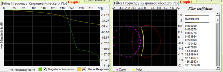
fig-2
6.Here we have taken sum of two sinusoidals of different frequencies (60Hz & 190Hz) as input so that user can easily understand the filter operation by choosing appropriate cutoff frequencies.
7.Graph 2 and 3 plots input and output signal respectively and also the corresponding frequency domain plots. Here we have given two radio buttons so that user can change from time domain to frequency domain plot.
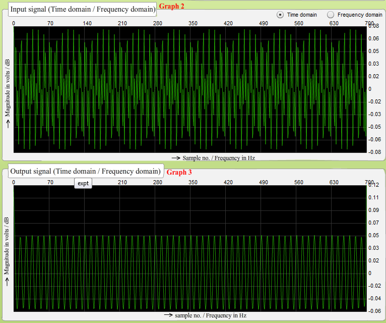
fig-3 Input and output signal time domain plots.

fig-4 Input and output signal frequency domain plots
8.Select lowpass filter and Butterworth filter design observe the filter frequency response, pole zero positions by changing cutoff frequency. Simultaneously see the output and compare with input signal. Write the discussion in the report portion of this experiment. Similarly change the filter design to remaining three types of designing techniques and change the cutoff frequency and observe the output.
9.Now change the passband ripple and stopband attenuation to another values and observe the results.
10.Repeat the step 8 and 9 for high pass also and observe the output signal and compare with input signal.
11.Use take snapshot button to take the screenshot of the experiment space
12.Complete the Observation and discuss the results in report generation.
13.Then click Yes I have finished my Experiment button to submit your report


Quizzes content.....

Video Lectures: